How to Find Standard Deviation of a Data Set: The Definitive Step-by-Step Guide

Understanding the spread of values within a data set is as crucial as analyzing their central tendency. Among the most vital tools for measuring variability is standard deviation—a statistical metric that quantifies how far individual data points deviate from the mean. Whether assessing student test scores, financial returns, or experimental measurements, calculating standard deviation transforms raw numbers into meaningful insights about data consistency and reliability.

This guide breaks down the precise steps to compute standard deviation, emphasizing clarity, accuracy, and practical application—essential for researchers, students, and data analysts alike.

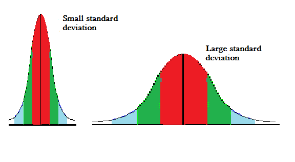
Standard deviation reveals the "average distance" of values from the mean, offering a quantitative measure of data dispersion. Unlike simple averages, which summarize central location, standard deviation captures the precision of data clustering.

As statistician Joseph Stein指出 in his foundational work, “Standard deviation is the most intuitive and widely used indicator of variability.” For any data set, accurate calculation of this value enables sound decision-making in fields ranging from quality control to risk assessment. The process, though mathematically grounded, is systematic and accessible when guided by clear steps.

Step-by-Step Method to Compute Standard Deviation

The calculation unfolds in predictable stages, each building upon the prior to yield a precise numerical result.

Mastering these stages ensures consistency and reproducibility, regardless of data size or format.

Step 1: Calculate the Mean of the Data Set

The starting point is the average of all values. Sum every observation and divide by the total count.

Mathematically: Mean (μ) = Σx / n where Σx is the sum of values, and n is the number of observations. Even a minor error here propagationly affects the entire result—precision in summation is nonnegotiable.

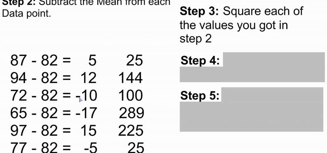
Step 2: Determine the Deviation of Each Value from the Mean

For each data point x, compute its deviation as (x − μ).

This transforms each value into how far it is from central tendency—positive deviations indicate over-mean values, negative ones under-mean. Their absolute magnitude captures distance, but signs preserve directional deviations.

Step 3: Square Each Deviation

Squaring ensures all deviations are positive and emphasizing larger differences.

For each deviation d, compute d². This step eliminates negative bias and amplifies outliers—key to sensing true variability rather than masking it.

Step 4: Compute the Variance

Variance measures the average squared deviation from the mean.

For a population: Variance (σ²) = Σ(x − μ)² / n For a sample, use: Sample Variance (s²) = Σ(x − x̄)² / (n − 1) The (n − 1) adjustment in sample variance corrects bias toward underestimating population spread—a nuance critical in inferential statistics.

Step 5: Take the Square Root to Obtain Standard Deviation

The final transformation from variance to standard deviation returns units consistent with original data, making interpretation immediate. For population: Standard Deviation (σ) = √σ² For sample: Standard Deviation (s) = √s² This step converts squared units into meaningful distance metrics, directly linking statistical analysis to real-world understanding.

Practical Examples: Applying the Calculation in Real World Contexts

Consider two data sets to illuminate the process:

Example 1: Daily Temperatures

Suppose daily temperatures over a week are: 68, 70, 72, 71, 69, 73, 70°F. Mean = (68+70+72+71+69+73+70)/7 = 70.43°F Deviations: −2.43, −0.43, 1.57, 0.57, −1.43, 2.57, 0.57 Squared deviations: 5.90, 0.18, 2.46, 0.32, 2.05, 6.60, 0.32 Sum = 17.73 → Variance (population) = 17.73 / 7 ≈ 2.53 → Standard Deviation = √2.53 ≈ 1.59°F This modest spread indicates consistent temperatures, reliable for climate reporting.

Example 2: Investment Returns

Returns (in %) over five years: 8, 12, 5, 10, 15.

Mean = (8+12+5+10+15)/5 = 10% Deviations: −2, 2, −5, 0, 5 → Squared: 4, 4, 25, 0, 25 Sum = 58 → Variance (population) = 58 / 5 = 11.6 → SD = √11.6 ≈ 3.41% Given the squared weights, even a single high return contributes significantly—standard deviation quantifies risk thus concretely, guiding portfolio decisions.

Key Considerations and Avoiding Common Pitfalls

While the method is systematic, accuracy hinges on careful execution: - Use population vs. sample variance appropriately—mixing formulas invalidates results.

- Verify arithmetic: even small miscalculations compound, especially with large data sets. - For unordered or skewed data, consider transformations or robust measures (e.g., interquartile range) to complement standard deviation. - In digital or spreadsheet environments, leverage built-in functions—Excel’s STDEV.P or STDEV.S—while understanding their underlying mechanics.

Calculators, Software, and calculator-verification

Modern tools drastically reduce manual computation errors. Spreadsheet formulas like STDEV.S automatically adjust for sample size via n−1, while statistical software packages automate variance and SD calculations with precision. Cross-checking hand-calculated results against software builds confidence, especially in high-stakes analyses.

Why Standard Deviation Remains Indispensable in Data Science

Standard deviation is far more than a statistical relic—it is foundational in modern data analysis. In quality assurance, low standard deviation signals consistent manufacturing output; high SD flags inconsistency requiring process adjustments. In finance, SD measures volatility—informing investment strategies and risk tolerance.

In scientific research, it contextualizes measurement precision, determining whether observed effects are significant or noise. Moreover, standard deviation underpins key statistical inferences. It quantifies confidence intervals, tests hypotheses via t-tests, and enables z-scores to standardize diverse datasets.

Without it, data would remain chaotic, inseparable from meaning.

The Power of Precision: How Standard Deviation Turns Numbers into Insights

Calculating standard deviation transforms a set of numbers into a narrative of consistency and variation. By quantifying how far data stray from the mean, it bridges raw observation with statistical truth.

From classrooms to boardrooms, from climate models to stock portfolios, standard deviation provides clarity in complexity. The methodology—simple in concept, rigorous in execution—remains one of statistics’ most enduring tools, empowering decision-makers with precision. Mastering its steps ensures not just accurate reports, but informed action grounded in data’s true pulse.