The Power of Parent Function Linear: A Foundational Force in Mathematics

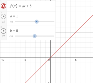
traces a quiet yet profound influence across every field relying on mathematical modeling—from economics and physics to engineering and data science. At its core, the parent function linear, defined by the form f(x) = mx + b, serves as the essential building block for understanding how relationships evolve predictably with constant rate of change. Unlike more complex functions that curve or oscillate, linear functions move steadily forward—or backward—along a straight line, capturing change in a way that is both intuitive and instantly actionable.

This unassuming linear model—where *m* represents slope (the dynamic force of change) and *b* denotes the y-intercept (the starting point)—pervades real-world applications. Its simplicity masks deep utility: once mastered, linear relationships empower learners and professionals alike to analyze trends, forecast outcomes, and make precise decisions. In essence, the linear function is not merely a mathematical concept; it is a gateway to logical reasoning about the world.

Unpacking the Structure: Understanding the Components of Linear Functions

At the heart of the parent function linear lies a clear, two-parameter architecture: slope and intercept. The slope, *m*, quantifies the rate of change—how much the output variable shifts in response to a one-unit increase in the input. A positive *m* signals growth, while a negative value reflects decline.

For example, in a budget projection, a slope of $50 per week represents the steady income added each week; over time, this linear pattern reveals total earnings with precision. The y-intercept, *b*, anchors the line on the vertical axis, representing the value of *f(x)* when *x* equals zero. This initial condition sets the starting context for any model—whether describing the baseline revenue before a sales campaign, the initial patient temperature in a medical study, or the at-rest voltage in an electrical circuit.

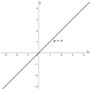
Together, *m* and *b* define a function’s behavior: - When *m* > 0: output rises steadily - When *m* < 0: output decays steadily - When *m* = 0: the function becomes constant at *b*, illustrating no change per unit *x* (a horizontal line). - When *b* = 0: the function passes through the origin, indicating symmetry and a direct proportionality between inputs and outputs. Understanding these components transforms abstract formulas into meaningful tools capable of decoding patterns in data and events.

Real-World Applications: Linear Functions in Action

Across disciplines, linear functions illuminate clear, actionable insights. In finance, linear models predict future investments using consistent interest rates or depreciation schedules. A $1,000 loan with a 5% annual interest rate follows f(x) = 1.05x — each year adding exactly 5% of the current value.

This predictability supports budgeting, risk assessment, and long-term planning. In transportation, speed and distance relationships are linear: distance traveled equals speed multiplied by time (d = vt). A car cruising at 60 miles per hour covers 60 miles in one hour, 120 in two — a straightforward linear progression where time drives distance steadily forward.

In environmental science, linear models track changes like temperature increase, where global averages rise at a roughly constant rate each decade. This helps scientists communicate trends clearly: “Global temperatures have increased by 1.1°C since pre-industrial times, at approximately 0.2°C per decade.” Engineers rely on linear approximations in stress-testing materials or signal processing, where inputs and outputs maintain proportional relationships under small variations. Even in everyday decisions—plotting weekly savings, managing inventory, or scheduling tasks—linear thinking underpins effective planning.

The Geometry of Linearity: Visualizing Slope and Intercept

Grasping linear functions becomes tangible through their graphical representation. On a coordinate plane, the linear equation *y = mx + b* traces a straight line whose steepness and direction reflect the slope, while its vertical position is determined by the intercept. - A steeper slope (*|m|* large) means faster change: a line rising sharply indicates rapid growth.

- A shallow slope suggests gradual shifts, while a negative slope reflects decline. - The y-intercept *b* determines where the line crosses the y-axis, anchoring the function’s base value. For example, plotting f(x) = 3x + 5 produces a line with a slope of 3 and y-intercept at (0, 5).

Each increase in *x* by 1 raises *y* by 3—and starting from *y = 5*, the function climbs predictably. Graphing multiple linear functions reveals intersections, trends, and divergences, offering visual clues about system behavior. This geometric clarity helps students and professionals alike interpret function behavior at a glance, identifying key transitions and determining critical values without lengthy calculations.

Predictive Power: Forecasting Trends with Linear Models

One of the most compelling strengths of the linear function lies in its predictive capability. Because outcomes evolve uniformly with each input increment, linear models serve as reliable tools for forecasting future states based on current trends. Consider utility pricing: a monthly phone plan charging $20 base plus $10 per data pack generates a total cost function f(x) = 10x + 20.

After three packs, the cost is $50; after ten, $120. This model projects accurate future bills, enabling users to anticipate expenses and plan budgets effectively. In epidemiology, early outbreak data often fits linear patterns—cases rising steadily in the initial stages—allowing health officials to estimate progression and allocate resources efficiently before exponential spikes occur.

Economists use linear models to project GDP growth, assuming stable annual increases. Retailers forecast seasonal demand with seasonal linear adjustments, optimizing inventory to meet anticipated sales. These applications highlight linearity’s role not just as description, but as a forward-looking instrument guiding action.

Calculations are straightforward: predicting *