Mastering Inverse Trigonometric Integrals: The Definitive Guide to Solving Complex Integrals

Inverse trigonometric integrals lie at the intersection of calculus, algebra, and geometric intuition, offering both a challenge and a gateway to deeper mathematical fluency. Far more than mechanical substitutions, these integrals demand strategic insight, recognizing key patterns, substitutions, and identities that unlock elegant solutions. This comprehensive guide reveals how to approach, transform, and solve inverse trigonometric integrals with precision—transforming confusion into confidence.

Whether you're preparing for exams, optimizing engineering models, or deepening your analytical toolkit, mastering these techniques is essential. With the right framework, even the most daunting integrals become routine.

The Core Principles of Inverse Trigonometric Functions in Integration

Understanding inverse trigonometric functions is foundational to mastering their integrals. These functions—arcsin(x), arccos(x), arctan(x)—are defined as the inverses of their respective trigonometric counterparts, with restricted domains that ensure single-valued outputs.

In integration, they appear as antiderivatives of rational, algebraic, and radical expressions involving square roots, often emerging in physical and applied contexts.

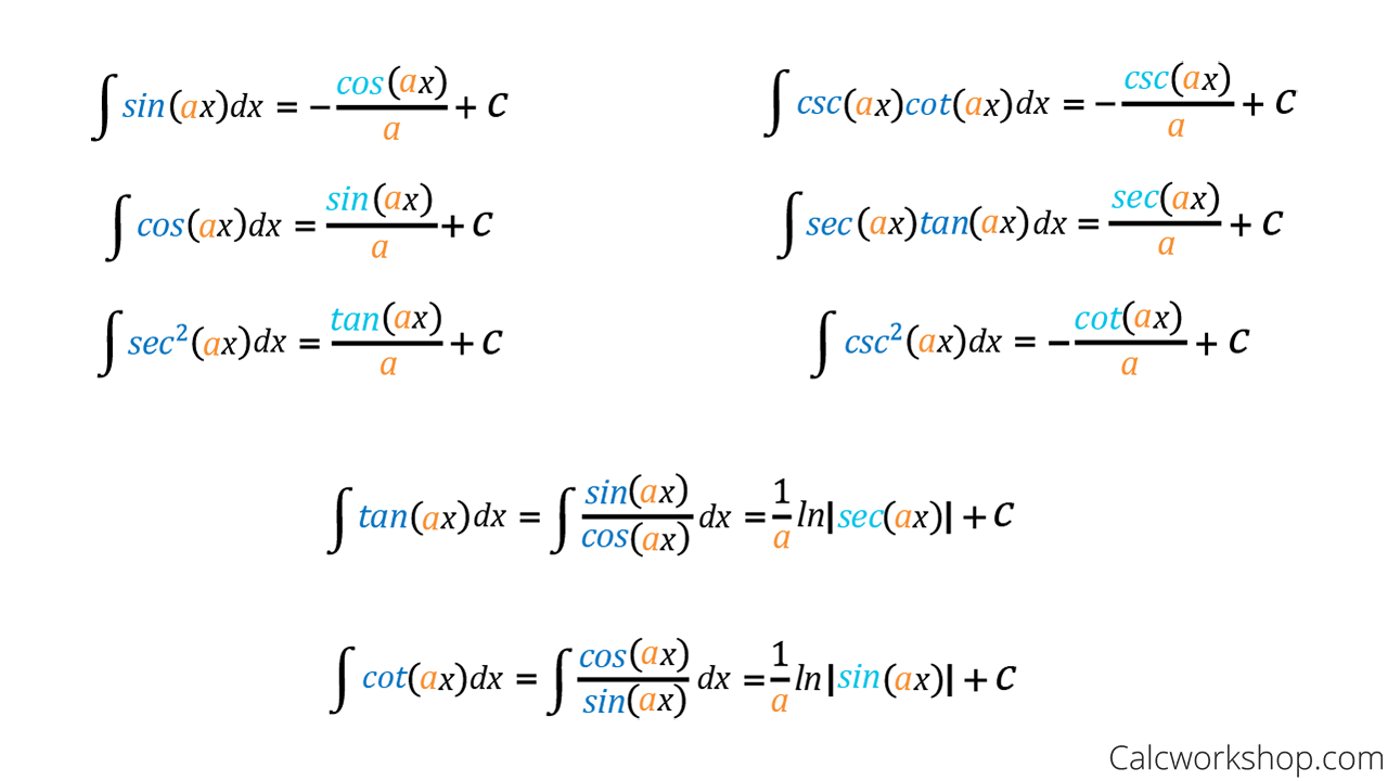
For derivatives, the chain rule reveals how trig derivatives influence integral forms: - d/dx [arcsin(x)] = 1 / √(1 – x²) - d/dx [arccos(x)] = –1 / √(1 – x²) - d/dx [arctan(x)] = 1 / (1 + x²) These derivatives not only inform differentiation but also guide substitution strategies—recognizing when a substitution like x = sin θ or x = tan θ simplifies the integral into a manageable form. Mastery begins with recognizing these standard patterns and their geometric interpretations.

Common Forms and Standard Techniques for Integration

Inverse trig integrals follow recurring structures, each respondable with a well-defined method.

Identifying these forms is the first step toward efficient solution. popular forms include:

The expressions ∫(ax + b)/√(p² – x²) and ∫√(p² – x²)/√(ax + b) appear frequently in calculus and physics. Here, standard techniques include trigonometric substitution—most effective when √(p² – x²) or similar radicals dominate the integrand.

For Example: ∫ dx / √(1 – x²) = arcsin(x) + C Demands substitution x = sin θ, transforming the radical into a trigonometric identity. Another common case: ∫ dx / (ax + b√(p² – x²)) benefits from rationalizing substitutions such as x = p sin θ, reducing complexity through geometric simplification.

Techniques such as partial fractions, manipulation of radicals via planned identities, and clever substitutions—like x = √(p² – u²) to handle √(p² – x²) terms—prove indispensable.

Recognizing these templates enables rapid, accurate integration.

Step-by-Step Method: Solving Inverse Trig Integrals

A systematic approach transforms abstract integrals into solvable problems. Follow this structured sequence: **Step 1: Identify the Integrand Type** Pinpoint whether the integrand includes linear expressions prefixing square roots, rational combinations, or pure inverse trigonometric functions. This inscription dictates the method.

**Step 2: Apply Key Substitutions** Use x = a sin θ for √(a² – x²), x = a tan θ for √(a² + x²), or x = a tanh u for expressions resembling √(x² + a²) in hyperbolic forms. **Step 3: Leverage Trigonometric and Algebraic Identities** Substitute the radical to simplify the integral, then apply Pythagorean identities to convert back to x. **Step 4: Simplify and Integrate** With reduced variables and simpler exponents, perform standard integration when applicable.

**Step 5: Substitute Back and Simplify** Replace utilities with original variables, simplifying logarithmic or algebraic expressions where necessary. Include constant of integration. Example: Solve ∫ sin⁻¹(x)/√(1 – x²) dx **Step 1**: Recognize √(1 – x²) suggests x = sin θ.

**Step 2**: Then dx = cos θ dθ, and √(1 – x²) = cos θ. The integral becomes ∫ (θ / cos θ) · cos θ dθ = ∫ θ dθ = (1/2)θ² + C = (1/2)arcsin²(x) + C. This straightforward path underscores how substitution dismantles complexity.

Advanced Techniques and Common Pitfalls

Beyond standard substitutions, seasoned practitioners deploy advanced tactics when conventional methods falter.

Logarithmic Results: Integrals involving rational inverses often yield natural logarithms—e.g., ∫ dx/(ax + b√(a² – x²)) results in ln|A + √(a² – x²)| / a + C. Recognizing this structure avoids algebraic overload.

Partial Fraction Decomposition Hybridization: When integrands combine inverse trig functions with rational polynomials, partial fractions combined with trigonometric identities streamline integration.

For instance, ∫ (ax + b)/[(x² + a²)√(x² + a²)] may split into rational and √(x² + a²) components before applying substitution.

African Forest Problem: Frequent trickery comes from misapplied substitutions—forgetting to account for Jacobian factors in multivariate settings or misidentifying domain restrictions. Precision in substitution domains prevents erroneous results. “A single misstep in θ’s range can invalidate the entire solution,” notes Dr.

Elena Torres, calculus theorist at MIT. “Understand the inverse function’s restricted domain.”

Applications in Science, Engineering, and Beyond

Inverse trig integrals are far more than academic exercises—they solve real-world challenges across disciplines.

• Physics: Arc length calculations, pendulum motion modeling, and electric potential integration rely on arcsin