How to Find Acceleration: Precision Methods Uncovered

Acceleration—often overlooked but fundamental to understanding motion—dictates how quickly speed changes over time, playing a pivotal role in everything from physics education to engineering design and sports performance. Obtaining accurate measurement of acceleration transforms raw data into actionable insight, enabling everything from safer vehicle dynamics to optimized athletic training. This article delivers a rigorous yet accessible guide to identifying and calculating acceleration, combining theoretical principles with practical tools and techniques used across science and industry.

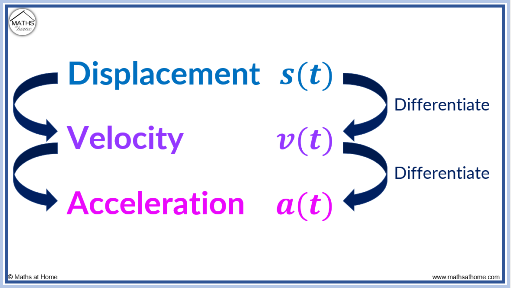
At its core, acceleration is defined as the rate of change of velocity with respect to time—mathematically expressed as a = Δv / Δt, where Δv is the change in velocity and Δt is the time interval. When an object’s speed increases, decelerates, or changes direction—even if constant in magnitude—its velocity vector varies, making acceleration the critical metric. Whether analyzing a car’s performance, biological locomotion, or mechanical systems, understanding how to measure this dynamic parameter ensures precise analysis and informed decision-making.

Step-by-Step Methods to Determine Acceleration

To accurately find acceleration, practitioners employ several established techniques, each suited to different contexts and data availability. The choice of method depends on access to tools, data quality, and the nature of the motion being studied.

The Accelerometer-Driven Approach

Modern digitized accelerometers, embedded in smartphones, wearables, or specialized sensors, provide the most direct means to measure acceleration.

These devices capture triaxial acceleration data—across x, y, and z axes—capturing both linear velocity changes and directional shifts in a single readout. Operating via piezoelectric, capacitive, or MEMS (micro-electromechanical systems) technology, accelerometers sample at high frequencies, producing detailed time-series data. Processing this data involves filtering noise, integrating acceleration to obtain velocity, and differentiating velocity to compute acceleration.

Während accelerometer output reflects proper acceleration—including gravity—correcting for gravitational components is essential when measuring true motion acceleration. In uniform gravitational fields, such as on Earth’s surface, gravity constrains vertical motion. Engineers and physicists often represent measured acceleration as a vector, distinguishing between gravitational and centripetal/momentum-driven components.

“Accelerometers have revolutionized motion analysis by making high-precision acceleration data accessible beyond labs,” notes Dr. Elena Torres, an applied physicist specializing in biomechanics. “With proper calibration and orientation, they deliver reliable readings in real time—critical for both research and field applications.”

Using Position and Velocity Data for Inverse Calculation

In scenarios where velocity and position data are known or can be reconstructed, acceleration can be computed indirectly using calculus-based formulas.

If position is recorded over time via GPS, camera tracking, or laser sensors and velocity is derived via finite differencing, acceleration follows naturally as the derivative of velocity with respect to time. For example, with discrete position measurements at intervals Δt, acceleration can be approximated using: i – v_i−1) / Δt where v_i denotes velocity between two time points. While this method is straightforward, it introduces error from timing inaccuracies and noise in position data.

To enhance reliability, filters and numerical integration techniques—such as Savitzky-Golay smoothing or Kalman filtering—are often applied before differentiation. Engineers frequently rely on this approach when high-frequency positional data is available, such as in robotics or vehicle navigation systems, where smooth trajectory modeling demands accurate acceleration estimates.

Velocity-Time Graph Analysis

Analyzing motion through velocity-time graphs offers a visually intuitive way to extract acceleration.

In a graphical representation, acceleration corresponds to the slope of the velocity curve; a changing slope indicates changing velocity, hence non-zero acceleration. For constant acceleration—common in uniformly accelerated motion—velocity changes linearly, producing a straight line with slope equal to acceleration. Stage 1: Plot velocity at sequential time points.

Stage 2: Fit a best-fit line using linear regression. Stage 3: The slope of this line yields constant acceleration.
Stage 4: For variable acceleration, divide small time intervals to compute instantaneous rates of change, effectively sampling acceleration across the motion timeline.

This method is especially valuable in educational settings and initial diagnostics, where visual interpretation aids understanding without complex instrumentation.

Practical Applications Across Disciplines

Acceleration measurement converges across scientific, engineering, and everyday domains, revealing its universal utility.

Automotive Safety and Performance Testing

Crash test dummies equipped with multi-axis accelerometers capture g-forces